Rocket Landing
Run this example at https://github.com/Trustworthy-AI/test-environments.
Rocket Landing
Background
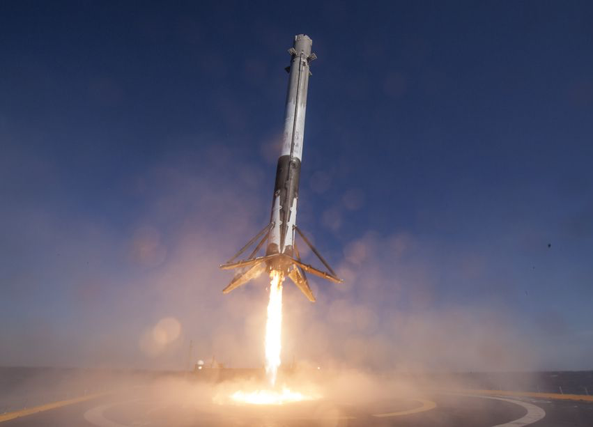
We now consider the problem of autonomous, high-precision vertical landing of an orbital-class rocket, a technology first demonstrated by SpaceX in 2015. In this experiment, the amount of thrust which the rocket is capable of deploying to land safely must be balanced against the payload it is able to carry to space; stronger thrust increases safety but decreases payloads. We consider two rocket designs and we evaluate their respective probabilities of failure (not landing safely on the landing pad) for landing pad sizes up to \(15\) meters in radius. That is, \(-f(x)\) is the distance from the landing pad's center at touchdown and \(\gamma=-15\). We evaluate whether the rockets perform better than a threshold failure rate of \(10^{-5}\).
We let \(P_0\) be the 100-dimensional search space parametrizing the sequence of wind-gusts during the rocket's flight.
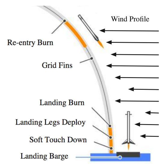
The booster thrusters correct for disturbances along the flight. The disturbances at every point in time follow a mixture of Gaussians. Namely, we consider 3 wind gust directions, \(w_1=(1,1,1)/\sqrt{3})\), \(w_2=(0,1,0)\), and \(w_3=(1,0,0)\). For every second in time, the wind follows a mixture: $$ W \sim \mathcal{N}(0,I) + w_1 B + w_2 \hat B + (1-\hat B)w_3, $$ where \(B \sim \text{Bernoulli}(1/3)\) and \(\hat B \sim \text{Bernoulli}(1/2)\). This results in 5 random variables for each second, or a total of 100 random variables since we have a 20 second simulation. The wind intensity experienced by the rocket is a linear function of height (implying a simplistic laminar boundary layer): \(f_w=CWp_3\) for a constant \(C\).
Implementation Details
We have created a python module that simulates this above scenario and connected it to the TrustworthySearch API with a simulation. There is a class to represent the rocket, and a function that calculates the mean distance from the center of the launch pad (which is where the rocket should ideally land).
SpaceCraft Module
The first step was to update the spacecraft files and functions from its TensorFlow source code (which was supplemental material for the NeurIPS Neural Bridge Simulation paper) to Pytorch. After verifying that the results of the final positions and gradients for the Pytorch version were the same as the original, we created the spacecraft into a module by adding an __init__ file.
Job Parameters
In this example we demonstrate a RISK job with parameters:
- Threshold = 15
- Stop Probability = 1e-5
- Stop Probability Confidence = .7
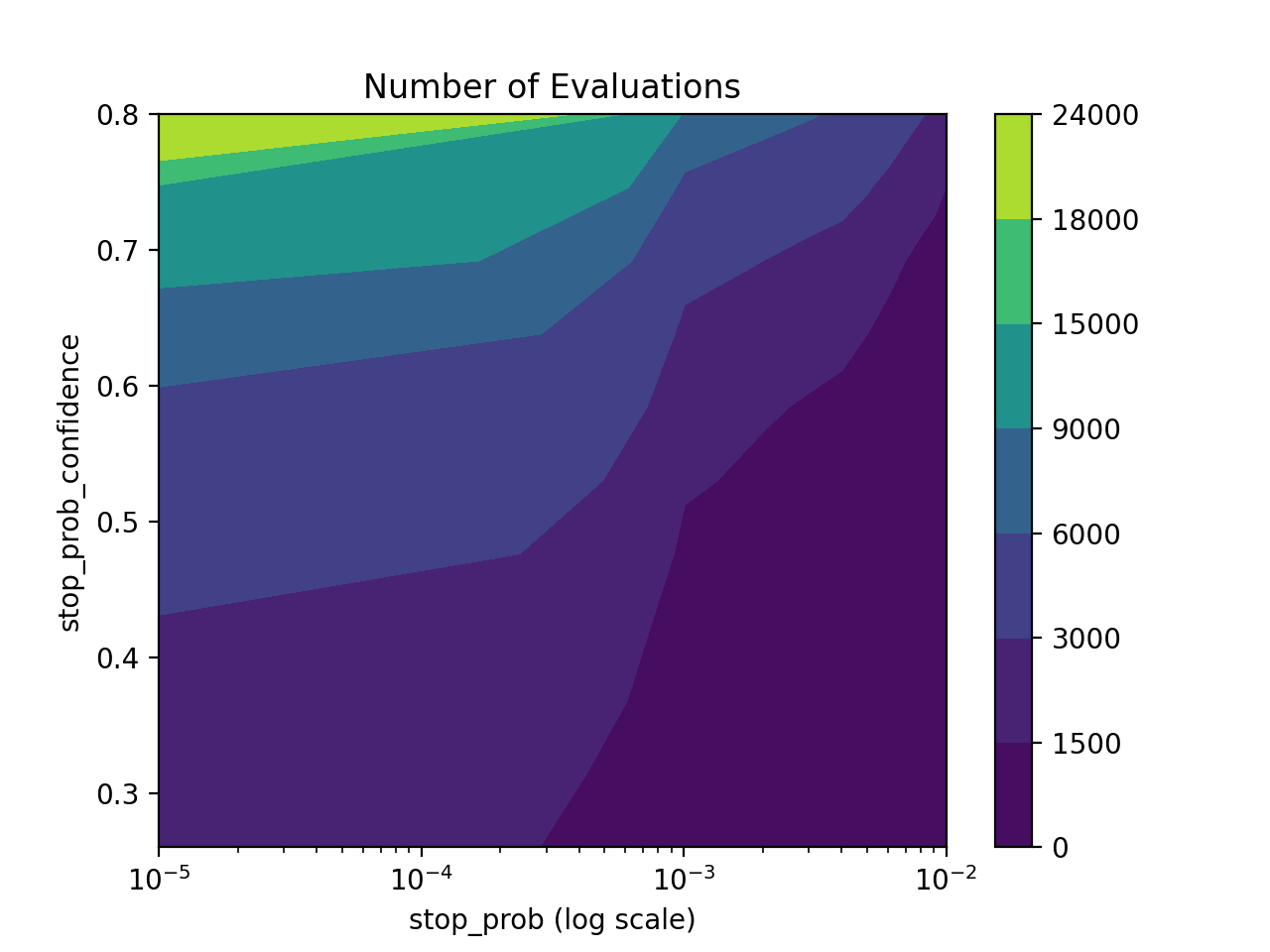
and collected the results to create a visualization of the parameters that made the simulation fail (e.g. made the rocket land far away from the launching pad). The threshold defines what objective values constitute a good/bad outcome, and stop_prob and stop_prob_confidence are used in order to calculate the number of evaluations needed. For our parameters we needed about 10500 evaluations. A contour plot is shown below in order to help better understand how these parameters affect the calculated number of evaluations:
When creating the job request, the dimension was 100, the dist_types was a list of 100 ts.Distribution.GAUSSIAN objects, and the job_mode was ts.JobStyle.Mode.MAXIMIZE. Note that as state above the job_type was ts.JobStyle.Type.RISK and thus the grid_density parameter did not affect anything. The first 60 gaussian objects of dist_types were the normal variables required for each simulation (3 per second with 20 seconds per simulation), the next 20 represented Bernoulli random variables with \(p=\frac{1}{3}\) and the final 20 represented Bernoulli random variables with \(p=\frac{1}{2}\). Since everything was given as normal distributions, we converted them to Bernoulli random variables by checking if it was less than the \(p^{th}\) quantile of the normal distribution.
Visualizations
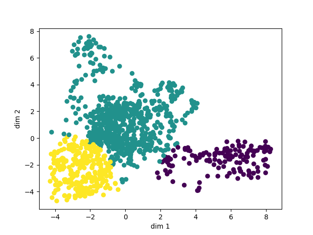
In order to visualize the parameters which made the simulation fail, we performed principal component analysis (PCA) on the parameters that had an objective of higher than 14. Using the Sci-Kit learn StandardScaler first to normalize the data, we reduced the dimension (which was originally 100 parameters) down to 2 dimensions. After this, we wanted to cluster the data, so we employed the silhouette method in order to find the optimal number of clusters for the data. The silhouette score used to evaluate each clustering is undefined when there is only 1 cluster, so to account for this case we used a heuristic saying if the max score is very bad (specifically below .4 as 1 is the max score indicating perfect fit and -1 is the lowest score) then that means the data is most likely in one big cluster. Additionally, we iteratively changed the cluster centers based on the points that had the smallest mahalanobis distance to them in order to improve the visualization. The parameters for the visualization are as follows:
- Threshold above which points are plotted = 14
- Max Number of Clusters Considered = 50
- Number of Iterations for Updating Centers = 30
- Error Tolerance for Early Stopping of Iterations for Updating Centers = .05
- Max silhouette_score to consider 1 cluster < .4
Below is an example plot clustered using the above method:
Additionally, it is useful to see at what probabilities the objective goes above a certain threshold, so we also created a plot of log-scale probabilites versus thresholds along with error bars. Below is an example of such a plot:
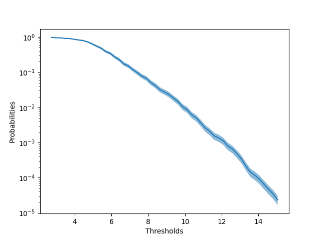
These visualizations should help the user understand more deeply under what conditions their job is failing.